🚀 AI for Backend Engineers: Building Intelligent Systems
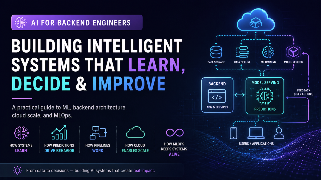
Backend engineering is evolving from static systems to intelligent systems.
As backend engineers, we are used to building systems that follow clear rules:
We define the logic.
The system executes it.
With Machine Learning, something fundamental changes:
The system can now learn patterns from data instead of relying entirely on explicitly programmed rules.
This is not simply an AI problem.
It is an architecture problem.
The moment Machine Learning enters a production backend, we need to think about:
- Data
- APIs
- Inference
- Latency
- Scalability
- Security
- Observability
- Model lifecycle
- Feedback loops
- Cloud infrastructure
This article connects Machine Learning + Backend Engineering + Cloud + MLOps from a production-system perspective.
🧭 From Rule-Based Systems to Learning Systems
Traditional backend systems are generally:
- Deterministic
- Rule-driven
- Explicitly programmed
- Relatively static after deployment
A simplified architecture looks like this:
flowchart LR
    A[Client Request] --> B[Backend API]
    B --> C[Business Rules]
    C --> D[Decision]
    D --> E[Response]
For example:
public boolean approveTransaction(Transaction transaction) {

    if (transaction.amount() > 10000) {
        return false;
    }

    if (!allowedCountry(transaction.country())) {
        return false;
    }

    return true;
}
This approach is predictable and easy to reason about.
But it also means that engineers must explicitly identify and encode the rules.
🤖 What Changes with Machine Learning?
A machine-learning system learns relationships from historical data.
Instead of manually encoding every rule:
flowchart LR
    A[Historical Data] --> B[Training Pipeline]
    B --> C[ML Model]
    C --> D[Inference Service]

    E[User Request] --> D
    D --> F[Prediction]
    F --> G[Backend Decision]
    G --> H[Response]
The system becomes data-driven.
A useful architectural principle is:
ML predicts → Backend decides
The model provides a prediction, probability, score, ranking, or representation.
The application can then apply business policy to that output.
⚡ Example: Fraud Detection
Consider a payment system.
A traditional fraud engine may use rules such as:
IF amount > threshold
AND country != expected_country
AND velocity > threshold
THEN flag_transaction
An ML system can learn fraud patterns from historical transactions.
flowchart LR
    A[Transaction Events] --> B[Data Pipeline]
    B --> C[Feature Engineering]
    C --> D[Fraud Model]
    D --> E[Risk Score]
    E --> F[Decision Service]

    F --> G[ALLOW]
    F --> H[REVIEW]
    F --> I[BLOCK]
The model might return:
The decision layer can then apply policy:
risk_score = model.predict_proba(features)[0][1]

if risk_score >= 0.90:
    decision = "BLOCK"
elif risk_score >= 0.60:
    decision = "REVIEW"
else:
    decision = "ALLOW"
Notice the separation:
This separation makes the system easier to test, govern, and evolve.
🧠 Supervised vs Unsupervised Learning
Supervised Learning
Supervised learning learns from labelled examples.
Typical applications:
- Fraud detection
- Spam detection
- Sentiment classification
- Credit-risk classification
- Customer churn prediction
Unsupervised Learning
Unsupervised learning works with unlabelled data and attempts to discover structure.
Typical applications:
- Customer segmentation
- Anomaly detection
- Behavioral analysis
- Pattern discovery
- Feature engineering
flowchart LR
    A[Unlabelled Data] --> B[Unsupervised Algorithm]
    B --> C[Clusters]
    B --> D[Anomalies]
    B --> E[Representations]
For backend engineers, the important point is:
Not every intelligent system starts with a predefined output label.
🎯 Classification vs Regression
Different ML problems produce different types of output.
| ML Problem | Output | Backend Example |
|---|---|---|
| Classification | Category | Fraud / Not Fraud |
| Regression | Numeric value | Risk Score |
| Clustering | Group | Customer Segment |
| Anomaly Detection | Outlier / Score | Suspicious Activity |
Classification
Regression
The backend can then use that output as part of a larger workflow.
🧩 A Simple ML Implementation
A backend engineer can start with a basic Scikit-Learn pipeline.
from sklearn.datasets import load_breast_cancer
from sklearn.model_selection import train_test_split
from sklearn.pipeline import Pipeline
from sklearn.preprocessing import StandardScaler
from sklearn.linear_model import LogisticRegression
from sklearn.metrics import accuracy_score

X, y = load_breast_cancer(return_X_y=True)

X_train, X_test, y_train, y_test = train_test_split(
    X,
    y,
    test_size=0.2,
    random_state=42,
    stratify=y
)

pipeline = Pipeline([
    ("scaler", StandardScaler()),
    ("model", LogisticRegression(max_iter=1000))
])

pipeline.fit(X_train, y_train)

predictions = pipeline.predict(X_test)

accuracy = accuracy_score(y_test, predictions)

print(f"Accuracy: {accuracy:.3f}")
The important part is not the specific algorithm.
It is the lifecycle:
flowchart LR
    A[Dataset] --> B[Split]
    B --> C[Preprocessing]
    C --> D[Training]
    D --> E[Evaluation]
    E --> F[Model Artifact]
🔌 Turning the Model into a Backend Capability
Once trained, the model can be exposed through an inference API.
A simplified FastAPI implementation:
from fastapi import FastAPI
from pydantic import BaseModel
import joblib

app = FastAPI()

model = joblib.load("model.joblib")


class PredictionRequest(BaseModel):
    features: list[float]


@app.post("/predict")
def predict(request: PredictionRequest):

    prediction = model.predict(
        [request.features]
    )[0]

    probability = model.predict_proba(
        [request.features]
    )[0].max()

    return {
        "prediction": int(prediction),
        "confidence": float(probability)
    }
The backend now exposes:
🏗️ Model Service vs Business Service
A common architecture mistake is to put business logic and model logic into one large service.
A cleaner separation is:
flowchart LR
    U[Client] --> G[API Gateway]

    G --> B[Business Service]

    B --> M[ML Inference Service]

    M --> P[Model Runtime]

    B --> DB[(Operational Database)]

    M --> O[Model Observability]
Business Service
Owns:
- Business workflows
- Authorization
- Domain rules
- Transactions
- Orchestration
ML Service
Owns:
- Model loading
- Feature transformation
- Inference
- Prediction
- Model-specific telemetry
This separation makes independent scaling and deployment easier.
🔁 ML Systems Are Pipelines, Not Just Models
A model is only one component in a larger system.
A production lifecycle may look like:
flowchart LR
    A[Data Sources] --> B[Ingestion]
    B --> C[Data Processing]
    C --> D[Feature Engineering]
    D --> E[Model Training]
    E --> F[Evaluation]
    F --> G[Model Registry]
    G --> H[Deployment]
    H --> I[Inference]
    I --> J[Monitoring]
    J --> K[Feedback]
    K --> A
This introduces engineering responsibilities around:
- Data ingestion
- Feature generation
- Model training
- Model validation
- Model deployment
- Inference
- Monitoring
- Feedback
- Retraining
- Version management
The model is part of the architecture, not the architecture itself.
🧠 Software Lifecycle vs ML Lifecycle
Traditional software often follows:
An ML system adds a learning loop:
Visually:
flowchart LR
    A[Production Traffic] --> B[Telemetry]
    B --> C[Data Pipeline]
    C --> D[Training]
    D --> E[Evaluation]
    E --> F[Deployment]
    F --> A
The key difference
Deployment is not the end of an ML system.
It is the beginning of a production feedback loop.
⚡ Real-Time Inference
Real-time ML runs inside the user request path.
Example:
User opens an application → recommendation service returns personalized results.
sequenceDiagram
    participant U as User
    participant API as Backend API
    participant R as Recommendation Service
    participant M as ML Model

    U->>API: Request
    API->>R: Recommendation Request
    R->>M: Predict / Rank
    M-->>R: Predictions
    R-->>API: Ranked Results
    API-->>U: Personalized Response
Real-time inference introduces:
- Latency requirements
- Throughput requirements
- Horizontal scaling
- Model loading
- Caching
- Failure handling
- Model versioning
🔄 Batch ML
Batch systems operate asynchronously.
Typical batch inputs include:
- Clicks
- Views
- Purchases
- Search behavior
- Transactions
- Application events
Architecture:
flowchart LR
    A[Events] --> B[Object Storage]
    B --> C[Batch Processing]
    C --> D[Feature Generation]
    D --> E[Training]
    E --> F[Evaluation]
    F --> G[Model Registry]
    G --> H[Production Model]
Batch processing is often simpler and cheaper when business requirements do not require immediate inference.
⚖️ Real-Time vs Batch
| Dimension | Real-Time | Batch |
|---|---|---|
| Latency | ms / seconds | minutes / hours |
| Cost | Higher | Usually lower |
| Complexity | Higher | Lower |
| Typical Use | Online decisions | Retraining |
| Response | Immediate | Delayed |
| Scaling | Continuous | Scheduled |
The important architecture question is:
What latency does the business actually require?
Not:
"Can we make everything real time?"
📈 Latency and System Complexity
A simplified relationship:
xychart-beta
    title "Relative System Complexity vs Latency Requirement"
    x-axis ["Batch", "Micro-Batch", "Near Real-Time", "Online Inference"]
    y-axis "Relative Complexity" 0 --> 100
    bar [20, 40, 65, 90]
As latency requirements become stricter, the architecture generally requires more operational sophistication.
This can introduce:
- Caching
- Dedicated inference services
- Accelerators
- Model optimization
- Asynchronous workflows
- Autoscaling
- High-availability design
🛍️ Recommendation System — A Complete Example
Recommendation systems are one of the clearest examples of ML integrated with backend and cloud architecture.
They combine:
- Backend APIs
- Event streams
- Data pipelines
- Feature engineering
- Ranking models
- Real-time inference
- Batch training
- Feedback loops
- Monitoring
End-to-End Architecture
flowchart TB
    U[Users] --> API[Backend API]

    API --> R[Recommendation Service]
    R --> M[Ranking Model]
    M --> API
    API --> U

    U --> E[User Events]

    E --> K[Event Bus]
    K --> D[Data Platform]

    D --> F[Feature Engineering]
    F --> T[Training Pipeline]
    T --> V[Model Evaluation]
    V --> MR[Model Registry]

    MR --> M

    R --> O[Inference Monitoring]
    O --> D
The same system is therefore performing two jobs:
                        Recommendation System
                                │
              ┌─────────────────┴─────────────────┐
              │                                   │
              ▼                                   ▼
       Real-Time Serving                     Continuous Learning
              │                                   │
              ▼                                   ▼
      User Experience                         Data Pipeline
              │                                   │
              ▼                                   ▼
          Prediction                            Training
              │                                   │
              └───────────────┬───────────────────┘
                              ▼
                       Better Recommendations
🧪 Model Evaluation
A model's output should not automatically be trusted.
For classification, common metrics include:
- Accuracy
- Precision
- Recall
- F1
- ROC-AUC
For regression:
- MAE
- MSE
- RMSE
- R²
Example:
from sklearn.metrics import (
    accuracy_score,
    precision_score,
    recall_score,
    f1_score
)

accuracy = accuracy_score(y_test, predictions)
precision = precision_score(y_test, predictions)
recall = recall_score(y_test, predictions)
f1 = f1_score(y_test, predictions)

print({
    "accuracy": accuracy,
    "precision": precision,
    "recall": recall,
    "f1": f1
})
The engineering question is:
Is the model good enough for the business decision?
A 95% accurate model may still be unacceptable for certain fraud, financial, medical, or security decisions if the cost of false negatives is extremely high.
📊 Model Version Comparison
Imagine a production team evaluating three model versions:
| Model | Precision | Recall | F1 |
|---|---|---|---|
| v1 | 0.88 | 0.81 | 0.84 |
| v2 | 0.91 | 0.86 | 0.88 |
| v3 | 0.93 | 0.89 | 0.91 |
Visual comparison:
xychart-beta
    title "F1 Score Across Model Versions"
    x-axis ["v1", "v2", "v3"]
    y-axis "F1 Score" 0 --> 1
    bar [0.84, 0.88, 0.91]
This makes model quality a measurable engineering signal rather than a one-time training result.
🔁 MLOps: The Continuous Loop
Production ML systems evolve continuously.
flowchart LR
    A[Collect Data] --> B[Validate Data]
    B --> C[Train]
    C --> D[Evaluate]
    D --> E[Register Model]
    E --> F[Deploy]
    F --> G[Monitor]
    G --> H[Detect Drift]
    H --> I[Retrain]
    I --> B
MLOps introduces practices around:
- Experiment tracking
- Model registry
- Data validation
- Model evaluation
- Automated deployment
- Monitoring
- Drift detection
- Retraining
- Rollbacks
⚠️ Production Challenges
| Challenge | Engineering Concern |
|---|---|
| Data Quality | Garbage-in / garbage-out |
| Data Drift | Input distribution changes |
| Model Drift | Prediction quality changes |
| Training/Serving Skew | Different transformations |
| Latency | Inference becomes too slow |
| Cost | Training/inference becomes expensive |
| Scaling | Traffic spikes |
| Observability | Hard-to-debug behavior |
| Versioning | Which model is serving? |
| Rollback | Safely revert bad models |
A useful architectural rule is:
Most production AI problems are system-level problems, not model-level problems.
🧠 What This Means for Backend Engineers
Backend engineers already understand:
- APIs
- Microservices
- Distributed systems
- Databases
- Caching
- Messaging
- Security
- Observability
- CI/CD
AI adds another layer:
flowchart LR
    A[Backend Engineering] --> D[Intelligent Systems]
    B[Machine Learning] --> D
    C[Cloud Engineering] --> D

    D --> E[Scalability]
    D --> F[Reliability]
    D --> G[Security]
    D --> H[Observability]
    D --> I[Continuous Learning]
The transition is not:
It can instead be:
flowchart LR
    A[Backend Engineering]
    B[Cloud Engineering]
    C[Machine Learning]

    A --> D[AI Engineering]
    B --> D
    C --> D

    D --> E[AI System Design]
    E --> F[Enterprise AI Architecture]
This is where backend experience becomes a strong foundation for AI engineering.
🏗️ Backend + ML + Cloud
A useful mental model:
                    Intelligent System
                           │
          ┌────────────────┼────────────────┐
          │                │                │
       Backend             AI              Cloud
          │                │                │
     APIs / Domain     Models / ML     Infrastructure
     Microservices     Inference       Scaling
     Events            Evaluation      Observability
          │                │                │
          └────────────────┼────────────────┘
                           │
                       Production
AI doesn't replace traditional engineering.
It extends it.
🛡️ Designing for Model Failure
A production backend should not necessarily fail completely because the model is unavailable.
A simple fallback pattern:
public RiskDecision evaluate(Transaction transaction) {

    try {
        double score = modelClient.predict(transaction);

        return decisionEngine.evaluate(score);

    } catch (ModelUnavailableException ex) {

        return fallbackDecision(transaction);
    }
}
This is the AI version of a familiar reliability principle:
Graceful degradation applies to AI systems too.
Other failure-handling patterns include:
- Timeouts
- Retries
- Circuit breakers
- Fallback models
- Cached predictions
- Rule-based fallback
- Asynchronous processing
🔐 Security Considerations
Introducing ML into a backend system also introduces new security concerns.
Examples:
Security must therefore cover:
- Training data
- Model artifacts
- Feature pipelines
- Inference APIs
- Credentials
- Access control
- Auditability
- Sensitive data
- Model endpoints
A production AI architecture should treat the model as part of the application's security boundary.
👀 Observability
Traditional backend observability often focuses on:
AI systems require additional signals:
Model latency
Prediction distribution
Confidence
Data drift
Feature drift
Model version
Evaluation metrics
Fallback rate
Inference errors
A conceptual observability architecture:
flowchart TB
    A[Application Metrics] --> O[Observability Platform]
    B[Infrastructure Metrics] --> O
    C[Inference Metrics] --> O
    D[Model Quality Metrics] --> O
    E[Data Drift Metrics] --> O
    F[Business Metrics] --> O

    O --> G[Dashboards]
    O --> H[Alerts]
    O --> I[Incident Response]
This is where traditional observability skills become even more valuable.
📐 AI System Design Perspective
When designing an AI-powered backend, ask:
1. What decision are we improving?
2. Is ML actually required?
3. What data is available?
4. What is the latency requirement?
5. What happens if the model is unavailable?
6. How will the model be evaluated?
7. How will drift be detected?
8. How will models be versioned?
9. How will the system scale?
10. How will the system be secured?
11. How will cost be controlled?
12. How will we know the system is actually improving?
This is the beginning of AI System Design.
📈 Static Systems → Intelligent Systems
The broader architectural evolution can be visualized as:
flowchart LR
    A[Rule-Based Systems]
    B[Data-Driven Systems]
    C[ML-Powered Systems]
    D[Generative AI Systems]
    E[Agentic Systems]
    F[Intelligent Enterprise Platforms]

    A --> B
    B --> C
    C --> D
    D --> E
    E --> F
The progression is:
Static Rules
      ↓
Data-Driven Decisions
      ↓
ML Predictions
      ↓
Generative AI
      ↓
AI Agents
      ↓
Intelligent Enterprise Systems
The backend engineer increasingly becomes an intelligent systems engineer.
🧭 Production Architecture Principles
1. Keep Business Logic Explicit
Do not hide critical deterministic business rules inside an opaque model when normal application logic is sufficient.
2. Treat Models as Dependencies
Models should have:
- Versions
- Health checks
- Monitoring
- Deployment strategy
- Rollback strategy
3. Separate Training from Inference
Training and inference normally have different:
- Compute requirements
- Scaling requirements
- Failure modes
- Deployment lifecycles
4. Design for Failure
Use:
5. Observe the Entire System
Monitor:
not just CPU and memory.
🧠 Final Takeaway
Machine Learning is not simply about algorithms.
It is about building systems that can:
- Learn from data
- Make intelligent predictions
- Support backend decisions
- Adapt to changing patterns
- Improve continuously over time
The architectural transition is:
And this is where traditional backend engineering starts evolving into AI System Design.
📚 Related Topics in the Enterprise AI Engineering Handbook
This article provides the engineering perspective.
For structured technical reference material, explore:
- Introduction to Machine Learning
- Machine Learning Fundamentals
- Machine Learning Lifecycle
- Machine Learning in Practice
- Machine Learning Ecosystem and Tools
🚀 What's Next?
This article is part of the:
AI for Backend Engineers
journey.
The broader path connects:
flowchart LR
    A[Machine Learning]
    B[Deep Learning]
    C[Generative AI]
    D[RAG]
    E[AI Agents]
    F[Agentic AI]
    G[AI System Design]
    H[Enterprise AI Architecture]

    A --> B
    B --> C
    C --> D
    D --> E
    E --> F
    F --> G
    G --> H
The goal is to understand how backend and cloud engineers can evolve toward designing and building production-grade intelligent systems.
💬 Final Thought
Backend engineering is evolving:
From static systems → intelligent systems.
And the engineers who can connect:
Data + Backend + Cloud + AI
will be well positioned to design the next generation of intelligent software systems.
🔗 Let's Connect
If you're exploring:
- AI Engineering
- Cloud AI Architecture
- MLOps
- Distributed ML Systems
- RAG & Agentic AI
- Scalable Backend Architecture
- AI System Design
💼 LinkedIn
https://www.linkedin.com/in/mihirkrjha/
📚 Enterprise AI Engineering Handbook
https://enterpriseai.handbook.mihirkjha.com/
📰 Enterprise AI Engineering Newsletter
https://www.linkedin.com/newsletters/enterprise-ai-engineering-7479222208079319041/
💻 GitHub
https://github.com/MihirKJha/enterprise-ai-blog
📌 Key Message
Build AI systems. Don't just build AI models.
For backend engineers:
Learn to design the system around the model.
© 2026 Mihir Jha