🚀 Deep Learning — The Foundation of Modern AI
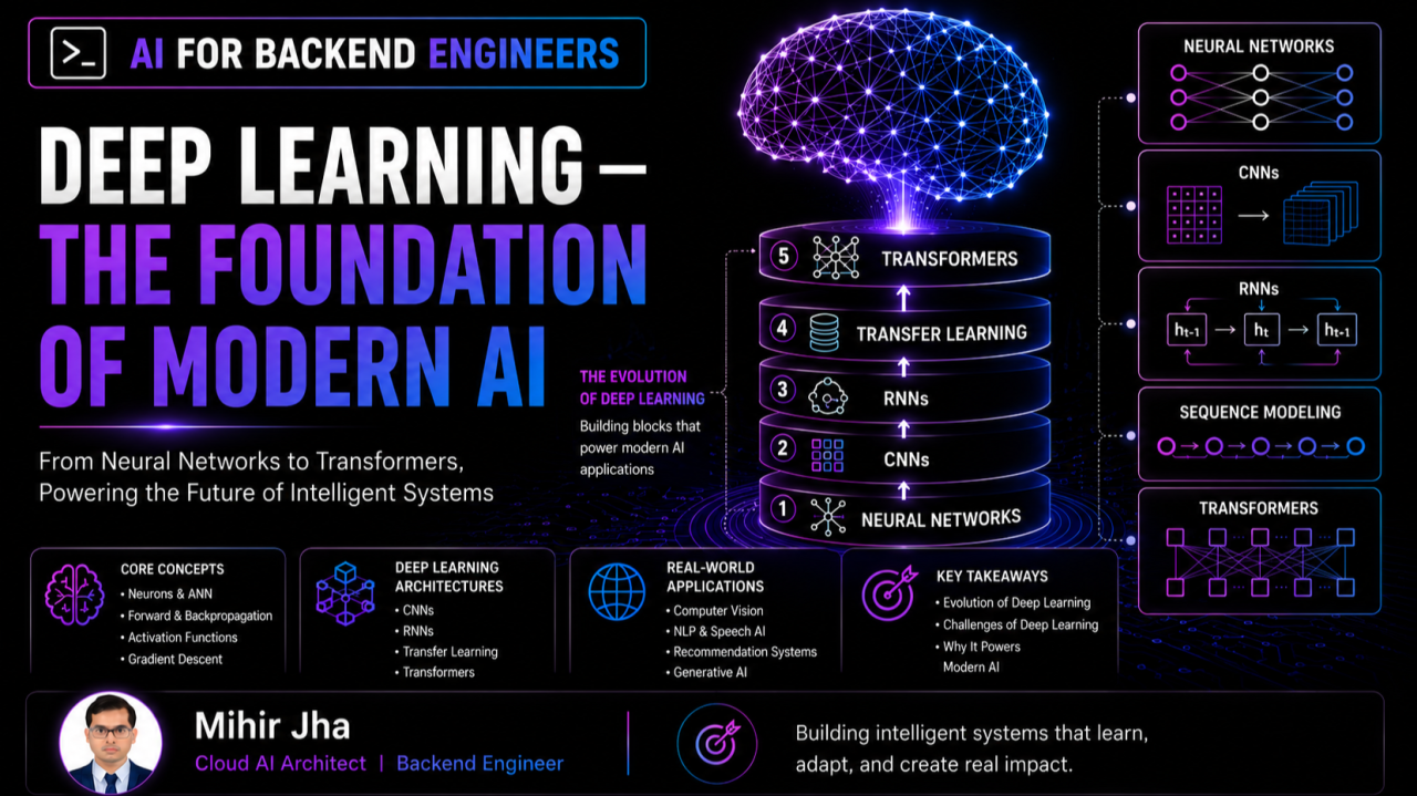
Deep Learning transformed AI by enabling systems to automatically learn complex representations from large amounts of data, providing the foundation for modern computer vision, speech, language, recommendation systems, and Generative AI.
Reading Time: 18–20 minutes
Difficulty: Intermediate
🎯 Learning Objectives
After reading this article, you will be able to:
- Understand why Deep Learning changed modern AI
- Explain the basic architecture of neural networks
- Understand how CNNs process image data
- Understand how RNNs process sequential data
- Explain the role of hidden state and sequence memory
- Understand why RNNs and LSTMs/GRUs faced scalability limitations
- Explain how Transfer Learning reduces training cost and data requirements
- Understand why Transformers became foundational to modern AI
- Understand how Deep Learning workloads run on cloud infrastructure
- Identify production challenges around cost, latency, scaling, and observability
- Connect Deep Learning concepts with backend and cloud architecture
🔥 Introduction
In the previous articles in the AI for Backend Engineers journey, we explored:
- Building intelligent systems
- Preparing data for Production AI
- Choosing the Right Machine Learning Algorithms
- Why AI Projects Fail in Production
We learned that:
- Data quality matters.
- Algorithm selection matters.
- Production AI requires continuous monitoring and improvement.
However, many modern AI applications require a level of pattern recognition that traditional Machine Learning often struggles to achieve.
Examples include:
- Image recognition
- Voice assistants
- Recommendation engines
- Natural Language Processing
- Generative AI
- Large Language Models
This is where Deep Learning changed everything.
Deep Learning enabled systems to automatically learn complex patterns and representations from large amounts of data instead of relying as heavily on manually engineered features.
The evolution can be viewed as:
Machine Learning
      │
      ▼
Neural Networks
      │
      ├── CNNs
      │
      ├── RNNs
      │     ├── LSTM
      │     └── GRU
      │
      ├── Transfer Learning
      │
      ▼
Transformers
      │
      ▼
Foundation Models
      │
      ▼
LLMs / Generative AI
      │
      ▼
RAG / AI Agents / Agentic AI
This article brings those concepts together and explains how they fit into real production systems — from model training to cloud infrastructure and operational challenges.
🧠 Why Deep Learning Changed AI
Traditional Machine Learning algorithms often depend heavily on manual feature engineering.
For example, a fraud detection system may require carefully designed features such as:
- Transaction amount
- Customer age
- Account history
- Merchant category
- Transaction frequency
The quality of these engineered features significantly influences model performance.
Deep Learning introduced a different approach.
Instead of manually defining every important feature, deep neural networks can learn increasingly useful representations directly from large amounts of data.
This enabled major advances in:
- Computer Vision
- Speech Recognition
- Natural Language Processing
- Recommendation Systems
- Generative AI
Traditional ML vs Deep Learning
| Dimension | Traditional ML | Deep Learning |
|---|---|---|
| Feature Engineering | Often extensive | Often learned automatically |
| Typical Data Volume | Small to medium | Medium to very large |
| Compute Requirements | Lower | Often significantly higher |
| Training Time | Usually shorter | Often longer |
| Model Complexity | Lower | Higher |
| Explainability | Often easier | Often more difficult |
| Image / Audio / Text | Task-dependent | Particularly strong |
| Production Infrastructure | Relatively simple | Often more complex |
The important point is not that Deep Learning replaces traditional Machine Learning everywhere.
Rather:
Deep Learning becomes particularly valuable when the underlying patterns are too complex or high-dimensional for manual feature engineering to be effective.
🔗 Neural Networks Explained for Engineers
At the heart of Deep Learning are Artificial Neural Networks (ANNs).
A neural network consists of interconnected layers that transform input data into predictions.
flowchart LR
    A[Input Layer] --> B[Hidden Layer 1]
    B --> C[Hidden Layer 2]
    C --> D[Hidden Layer 3]
    D --> E[Output Layer]
Input Layer
The input layer receives raw or prepared data.
Examples:
- Numerical features
- Image pixels
- Text representations
- Audio features
- Sensor measurements
Hidden Layers
Hidden layers learn representations and relationships within the input.
As networks become deeper, later layers can learn increasingly complex representations.
Output Layer
The output layer produces the final prediction.
Examples:
- Class probability
- Regression value
- Next token probability
- Image classification
- Anomaly score
🔄 How Neural Networks Learn
A neural network learns through an iterative optimization process.
A simplified flow is:
Input Data
    │
    ▼
Forward Propagation
    │
    ▼
Prediction
    │
    ▼
Loss Calculation
    │
    ▼
Backpropagation
    │
    ▼
Weight Updates
    │
    ▼
Repeat
Forward Propagation
Data flows from the input layer through the network to produce a prediction.
Loss Calculation
The prediction is compared with the expected target using a loss function.
Backpropagation
The error signal is propagated backward through the network.
Optimization
An optimizer updates model parameters to reduce the loss.
This process repeats over many training iterations.
💻 Simplified Neural Network Example
A simple neural network can be expressed with Keras like this:
from tensorflow import keras
from tensorflow.keras import layers

model = keras.Sequential([
    layers.Input(shape=(10,)),
    layers.Dense(64, activation="relu"),
    layers.Dense(32, activation="relu"),
    layers.Dense(1, activation="sigmoid")
])

model.compile(
    optimizer="adam",
    loss="binary_crossentropy",
    metrics=["accuracy"]
)
The code is simple, but production engineering introduces additional questions:
- Where does the training data come from?
- How are features versioned?
- How is the model evaluated?
- Where is the trained model stored?
- How is inference exposed?
- How is latency monitored?
- How is model drift detected?
Again, the model is only one component of the larger system.
📷 CNNs — Powering Computer Vision
Convolutional Neural Networks (CNNs) transformed image processing and computer vision.
Traditional fully connected neural networks treat input features largely as independent values.
CNNs instead exploit local spatial relationships in images.
They can automatically learn hierarchical visual representations.
The progression often looks like:
This ability made CNNs foundational to many computer vision systems.
🧩 How a CNN Processes an Image
A simplified CNN architecture can be represented as:
flowchart LR
    A[Input Image] --> B[Convolution]
    B --> C[ReLU]
    C --> D[Pooling]
    D --> E[Convolution]
    E --> F[ReLU]
    F --> G[Pooling]
    G --> H[Flatten]
    H --> I[Fully Connected Layer]
    I --> J[Output]
1. Input Layer
The input layer receives an image as a matrix of pixel values.
Examples:
2. Convolution Layer
A convolution layer applies small filters, also called kernels, across an image.
These filters learn patterns such as:
- Edges
- Corners
- Lines
- Textures
During training, useful filters are learned automatically.
3. Activation Layer
An activation function introduces non-linearity into the network.
A common activation is ReLU — Rectified Linear Unit.
This allows the network to model more complex relationships.
4. Pooling Layer
Pooling reduces the spatial dimensions of feature maps.
Common approaches include:
- Max Pooling
- Average Pooling
Benefits can include:
- Reduced computation
- Lower memory consumption
- Greater spatial robustness
- Reduced feature-map size
5. Fully Connected Layer
After feature extraction, learned representations are flattened and passed to one or more dense layers for decision making.
6. Output Layer
The output layer produces the final prediction.
Examples:
- Cat vs Dog
- Tumor detection
- Vehicle recognition
- Object classification
Typical output activations include:
- Sigmoid → Binary classification
- Softmax → Multi-class classification
- Linear → Regression
🏥 CNN Real-World Applications
CNN-based systems have been used across many industries.
Healthcare
- X-ray analysis
- CT image analysis
- MRI analysis
- Pathology image analysis
Manufacturing
- Automated defect detection
- Quality inspection
- Visual anomaly detection
Retail
- Visual search
- Product recognition
- Image-based classification
Autonomous Systems
- Traffic-sign recognition
- Pedestrian detection
- Lane detection
- Object recognition
Consumer Applications
- Face unlock
- Photo tagging
- OCR
- Augmented reality
CNNs remain an important foundation for visual AI systems, even as newer architectures such as Vision Transformers have become increasingly important.
⏳ RNNs — Powering Sequential Intelligence
While CNNs transformed computer vision, many real-world problems involve sequential data.
Examples include:
- Text
- Speech
- Time-series data
- Sensor readings
- User activity streams
In these problems, the order of information matters.
For example:
"I love AI"
is not equivalent to:
"AI loves me."
Traditional feed-forward neural networks do not naturally maintain a memory of previous inputs.
This is where Recurrent Neural Networks (RNNs) became important.
🧠 How RNNs Process Sequential Data
Unlike feed-forward neural networks, RNNs maintain a hidden state that carries information from previous time steps.
flowchart LR
    A[x1] --> B[RNN Cell]
    B --> C[h1]
    C --> D[RNN Cell]
    E[x2] --> D
    D --> F[h2]
    F --> G[RNN Cell]
    H[x3] --> G
    G --> I[h3]
    I --> J[Output]
At each time step, the model combines:
- Current input
- Previous hidden state
to generate:
- Updated hidden state
- Current output
🔄 RNN Processing Model
A simplified flow is:
Input at t1
   │
   ▼
RNN Cell
   │
   ▼
Hidden State
   │
   ├──────────────┐
   │              ▼
   │         Input at t2
   │              │
   └──────────► RNN Cell
                  │
                  ▼
              Hidden State
                  │
                  ▼
               Input at t3
                  │
                  ▼
               RNN Cell
                  │
                  ▼
                Output
The same cell and weights are reused across time steps.
This allows the model to learn temporal relationships.
💬 Example: Language Sequence
Consider:
The prediction depends not only on the current token but also on the context accumulated from previous tokens.
The same idea can apply to:
- Speech recognition
- Time-series forecasting
- Predictive maintenance
- Sensor streams
- User behavior analysis
⚠️ RNN Limitations
Although RNNs introduced memory into neural networks, they struggled with long sequences.
Important challenges included:
- Vanishing gradients
- Difficulty learning long-term dependencies
- Sequential computation
- Slower training
These challenges motivated architectures such as:
- LSTM
- GRU
LSTMs and GRUs improved the ability to model long-term dependencies, but sequential processing remained a limitation for large-scale training.
That limitation eventually contributed to the rise of the Transformer architecture.
🚀 Transfer Learning — Building AI Faster and Smarter
Training a Deep Learning model from scratch can be expensive, time-consuming, and data-intensive.
Organizations may need:
- Large labelled datasets
- GPU infrastructure
- Long training cycles
- Significant engineering effort
For many business problems, this is not practical.
This is where Transfer Learning became extremely valuable.
Instead of learning everything from scratch, a model can reuse knowledge learned from a large source dataset and adapt it to a related task.
A useful analogy for software engineers is:
Transfer Learning is similar to reusing a mature library or framework instead of rebuilding the same capability from scratch.
🔄 How Transfer Learning Works
flowchart LR
    A[Large Source Dataset] --> B[Pre-trained Model]
    B --> C[Reusable Representations]
    C --> D[Fine-Tuning]
    D --> E[Business-Specific Model]
    E --> F[Production Deployment]
1. Large Source Dataset
A model is trained on a large dataset.
Examples may include:
- ImageNet
- Large text corpora
- Large speech datasets
2. Pre-trained Model
The model learns general representations.
Examples:
- Image features
- Language representations
- Speech patterns
3. Fine-Tuning
The model is adapted using a smaller domain-specific dataset.
Depending on the use case, engineers may:
- Freeze early layers
- Train later layers
- Fine-tune the full model with a smaller learning rate
4. Business-Specific Model
The adapted model becomes specialized for a specific task.
Examples:
- Medical image classification
- Manufacturing inspection
- Product classification
- Document analysis
- Domain-specific text classification
5. Production Deployment
The trained model is deployed through:
- APIs
- Applications
- Batch pipelines
- Cloud AI platforms
💡 Transfer Learning Example
Imagine building an AI system to detect manufacturing defects.
Training a vision model from scratch may require a very large labelled dataset.
Instead, engineers can start with a pre-trained model that has already learned visual representations such as:
- Edges
- Shapes
- Textures
- Objects
The model can then be adapted to recognize manufacturing defects.
Potential advantages include:
- Faster development
- Lower training cost
- Smaller domain-specific dataset requirements
- Faster experimentation
☁️ Transfer Learning and Modern AI
Transfer Learning is now a core pattern throughout modern AI.
It appears in:
- Computer Vision
- NLP
- Speech
- Multimodal AI
- Foundation Models
- LLM adaptation
Modern organizations often build on pre-trained models instead of starting from random initialization.
This becomes especially important as model sizes increase.
🤖 Transformers — The Foundation of Modern AI
Perhaps the most significant architectural breakthrough in modern AI is the Transformer.
CNNs transformed computer vision.
RNNs enabled sequence modeling.
Transformers introduced a more scalable approach to understanding relationships across sequences.
The key innovation is the Attention mechanism.
❓ Why RNNs Were Not Enough
Although RNNs, LSTMs, and GRUs improved sequence modeling, they still faced limitations.
Long-Term Dependencies
As sequences become longer, important information from earlier positions can become harder to preserve.
Sequential Processing
RNNs process information step by step.
This limits parallelism during training.
Scalability
Large-scale training becomes increasingly expensive when the architecture depends heavily on sequential computation.
Researchers needed an architecture that could process sequences more efficiently while learning relationships between distant elements.
⚡ The Transformer Revolution
Transformers changed the approach.
Instead of processing information sequentially through recurrence, Transformers use attention mechanisms to model relationships across the sequence.
Conceptually:
RNN:

Token 1 → Token 2 → Token 3 → Token 4
   │         │         │         │
 Hidden    Hidden    Hidden    Hidden
 State     State     State     State


Transformer:

Token 1 ─────────┐
Token 2 ─────────┤
Token 3 ─────────┼──► Attention ──► Representation
Token 4 ─────────┘
This approach enables substantially more parallel computation during training.
🧠 Attention at a High Level
Attention allows a model to determine which parts of an input sequence are more relevant to another part of the sequence.
For example:
Instead of relying only on a sequential hidden state, attention allows the model to learn relationships between elements.
A simplified representation is:
flowchart LR
    A[Input Tokens] --> B[Query]
    A --> C[Key]
    A --> D[Value]

    B --> E[Attention Scores]
    C --> E

    E --> F[Weighted Values]
    D --> F

    F --> G[Contextual Representation]
We will explore Self-Attention, Query-Key-Value representations, Encoder/Decoder architectures, BERT, GPT, and modern LLMs in subsequent articles.
🌍 Why Transformers Matter
Transformers became foundational to many modern AI systems.
They power or underpin technologies used for:
- Large Language Models
- Generative AI
- Machine Translation
- AI Assistants
- Code Generation
- Intelligent Search
- Document Intelligence
- Multimodal AI
- Vision Transformers
- Speech AI
The evolution can be summarized as:
Neural Networks
      ↓
CNNs / RNNs
      ↓
LSTM / GRU
      ↓
Transformers
      ↓
Foundation Models
      ↓
LLMs / Generative AI
      ↓
RAG / AI Agents / Agentic AI
🏢 Transformers in Production
Modern organizations generally do not train large foundation models entirely from scratch.
Instead, many systems rely on:
- Pre-trained foundation models
- Fine-tuning or adaptation
- Retrieval
- Prompting
- Tool integration
- Managed inference platforms
Production Transformer-based systems can support:
Enterprise Search
Retrieval and question answering across company knowledge.
AI Assistants
Conversational support and workflow assistance.
Document Intelligence
Extraction, summarization, classification, and reasoning over documents.
Customer Support
Automated response generation and assistance for support agents.
Code Generation
Developer copilots and software-development assistance.
Knowledge Management
Search, summarization, and knowledge extraction.
🏗️ Transformer Production Architecture
A simplified production architecture can look like:
flowchart LR
    A[User / Application] --> B[API Gateway]
    B --> C[AI Application Service]

    C --> D[Prompt / Context Construction]
    D --> E[Transformer / LLM]

    E --> F[Response]
    F --> G[Application]

    C --> H[Observability]
    C --> I[Security]
    C --> J[Cost Controls]
In modern AI applications, this architecture expands further to include:
- Retrieval
- Vector stores
- Tool calling
- Guardrails
- Evaluation
- Caching
- Model routing
- Human review
These become major architecture topics in the upcoming RAG and Agentic AI phases.
☁️ Deep Learning on Cloud Infrastructure
Deep Learning workloads often require significant computational resources.
Traditional CPUs may not be sufficient for large-scale training.
Modern workloads rely heavily on:
- GPUs
- Specialized accelerators
- Distributed training infrastructure
- High-throughput storage
- High-bandwidth networking
AWS
Examples include:
- SageMaker Training Jobs
- EC2 GPU instances
Microsoft Azure
Examples include:
- Azure Machine Learning compute
- Azure GPU virtual machines
Google Cloud
Examples include:
- Vertex AI Training
- TPU infrastructure
- GPU-based training environments
☁️ Cloud Deep Learning Architecture
A simplified architecture:
flowchart LR
    A[Training Data] --> B[Cloud Storage]
    B --> C[Training Pipeline]

    C --> D[GPU / TPU Cluster]
    D --> E[Model Artifacts]

    E --> F[Model Registry]
    F --> G[Deployment]

    G --> H[Inference API]
    H --> I[Applications]

    G --> J[Monitoring]
    J --> K[Feedback]
    K --> C
Cloud platforms allow organizations to scale Deep Learning workloads without purchasing and maintaining all underlying hardware themselves.
📊 Production Challenges in Deep Learning
While Deep Learning unlocks powerful capabilities, it also introduces operational challenges.
High Infrastructure Cost
Large training workloads can require significant GPU resources.
Long Training Times
Complex models can require hours, days, or longer training cycles.
Explainability Challenges
Understanding why a model produced a particular decision can be difficult.
Monitoring Complexity
Model quality can degrade even when infrastructure appears healthy.
Large Model Sizes
Larger models can increase:
- Memory usage
- Inference latency
- Infrastructure cost
- Deployment complexity
Production systems therefore require a balance between:
Performance + Cost + Scalability + Reliability + Maintainability
⚠️ Common Mistakes Teams Make
Organizations can struggle when they:
- Train unnecessarily large models
- Ignore infrastructure costs
- Skip monitoring and observability
- Overlook latency requirements
- Fail to leverage transfer learning
- Focus on model complexity instead of business value
- Deploy without a clear rollback strategy
- Underestimate inference infrastructure requirements
The best Deep Learning system is not necessarily the largest.
It is the system that reliably delivers business value within its production constraints.
📦 Deep Learning Production Checklist
Before deploying a Deep Learning workload, consider:
| Area | Key Question |
|---|---|
| Data | Is the training data representative? |
| Model | Does the model generalize? |
| Compute | Is the GPU/accelerator strategy appropriate? |
| Latency | Does inference meet the required SLA? |
| Cost | Is the model economically viable? |
| Scaling | Can inference scale with demand? |
| Monitoring | Can degradation be detected? |
| Security | Are models and data protected? |
| Governance | Are compliance requirements satisfied? |
| Rollback | Can model versions be safely reversed? |
🚀 In One Minute
- Neural Networks learn complex patterns from data.
- CNNs became foundational for computer vision.
- RNNs introduced sequence memory.
- LSTM and GRU improved long-term sequence modeling.
- Transfer Learning enabled reuse of pre-trained knowledge.
- Transformers changed scalable sequence modeling.
- Transformers became foundational to modern Generative AI.
- Cloud platforms provide scalable GPU and accelerator infrastructure.
- Production Deep Learning requires monitoring, optimization, security, and cost management.
🎯 Final Takeaway
Deep Learning has become the engine behind many of today's AI breakthroughs.
From:
- Image recognition
- Speech processing
- Recommendation systems
- Natural Language Processing
- Generative AI
- Large Language Models
deep neural networks have enabled capabilities that were previously difficult or impractical.
However, production success requires far more than powerful models.
It requires:
Quality Data + Scalable Infrastructure + Monitoring + Cost Management + Cloud-Native Architecture
For software and backend engineers, the key is not simply understanding how a neural network works.
The real opportunity is understanding how the model becomes part of a reliable production system.
🧠 From Deep Learning to AI Engineering
The progression we have covered is:
flowchart LR
    A[Machine Learning] --> B[Deep Learning]
    B --> C[Neural Networks]
    C --> D[CNNs / RNNs]
    D --> E[Transfer Learning]
    E --> F[Transformers]
    F --> G[Foundation Models]
    G --> H[LLMs]
    H --> I[RAG]
    I --> J[AI Agents]
    J --> K[Agentic AI]
This progression is important because modern AI applications are not disconnected technologies.
They are layers built on top of foundational concepts.
📚 Related Enterprise AI Engineering Handbook Topics
For structured, chapter-based learning, continue with the Enterprise AI Engineering Handbook:
- Deep Learning Fundamentals
- Neural Networks
- CNNs
- RNNs
- Transfer Learning
- Transformers
- Foundation Models
- Large Language Models
Update the chapter URLs above to the exact paths used in your current handbook
mkdocs.yml.
🔮 What's Next
So far in the AI for Backend Engineers journey, we have explored:
- Machine Learning Fundamentals
- Data Preparation
- ML Algorithms
- Production ML Challenges
- Deep Learning
The next major transition is into:
Large Language Models & Foundation Models
We will explore questions such as:
- What exactly is a Large Language Model?
- Why was the Transformer architecture revolutionary?
- What is Self-Attention?
- How are BERT and GPT different?
- How do LLMs generate text?
- Why do LLMs hallucinate?
- How do embeddings work?
- How are LLMs integrated into production systems?
Understanding these concepts provides the foundation for the next stages:
LLMs → RAG → AI Agents → Agentic AI
📚 AI for Backend Engineers — Learning Journey
✅ Building Intelligent Systems
        ↓
✅ Preparing Data for Production AI
        ↓
✅ Choosing the Right Machine Learning Algorithms
        ↓
✅ Why AI Projects Fail in Production
        ↓
✅ Deep Learning — The Foundation of Modern AI
        ↓
⏭️ Large Language Models in Real Systems
        ↓
RAG
        ↓
AI Agents
        ↓
Agentic AI
        ↓
AI System Design
        ↓
Production Enterprise AI
🔗 Let's Connect
If you're exploring:
- AI Engineering
- Cloud AI Architecture
- MLOps
- Distributed ML Systems
- RAG & Agentic AI
- Scalable Backend Architecture
- AI System Design
Let's connect and learn together.
🔗 LinkedIn:
https://www.linkedin.com/in/mihirkrjha/
📰 Enterprise AI Engineering Newsletter:
https://www.linkedin.com/newsletters/enterprise-ai-engineering-7479222208079319041/
📚 Enterprise AI Engineering Handbook:
https://enterpriseai.handbook.mihirkjha.com/
💻 GitHub:
https://github.com/MihirKJha/enterprise-ai-blog
👨💻 About the Author
Mihir Jha
Software Architect | AI Engineering | Cloud Architecture | Backend Engineering
I focus on bridging traditional software and cloud engineering with modern AI engineering to design scalable, secure, observable, and production-ready intelligent systems.